In ancient Greece, philosophers believed that celestial bodies moved in perfect circles with uniform velocity. When observations disagreed with this simple circular motion, the astronomers created complicated models containing combinations of many circles. They were able to decrease the difference between their models and the observations, but never made a perfect match.

Despite this failure, astronomers in Europe continued to adhere to the ancient assumption that heavenly motions must always be circular with a constant velocity. The greatest of the Renaissance observers, Tycho Brahe, was unable to devise any model which could match the thousands of careful measurements he gathered during decades of work. After his death, the astronomer Johannes Kepler, who had moved to Prague to work for Tycho and succeeded him as the imperial mathematician of the Holy Roman Empire, continued to work on models of the Solar System. He, too, failed to devise a model with purely circular motions which could account for the observations.

Kepler, unlike his predecessors, had a vast archive of precise measurements. His confidence in the data was strong enough that he finally cast aside the notion that all celestial motions must be perfect circles. When he allowed the planets to move in ellipses, not circles, he finally was able to match the data; that was Kepler's First Law: "the planets move in elliptical orbits, with the Sun at one focus."

This by itself wasn't enough; Kepler also discovered that the velocity of the planets must change as they move around the Sun: increasing as they come closer, decreasing as they retreat. Was there any way to describe this variation in velocity mathematically? Yes! Kepler put forth his solution in his Second Law: "a line from a planet to the Sun sweeps over equal areas in equal intervals of time."

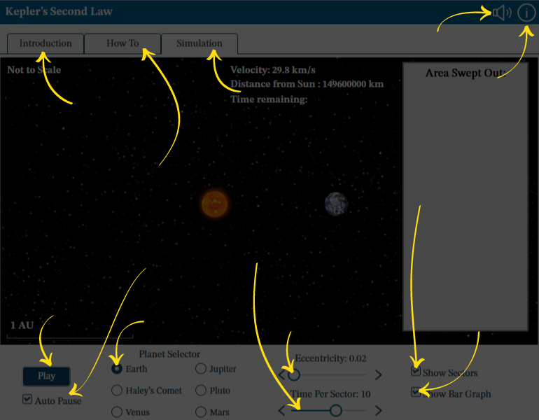
This interactive shows you Kepler's Second Law in action. In the interests of clarity, the size of the Sun and planets are all exaggerated relative to their orbital sizes.

You will explore Kepler's 2nd law, seeing how a planet's speed changes in different parts of an elliptical orbit.

To make it easier to compare orbits with different eccentricities (more or less elliptical), all the orbits have the same semi-major axis (width): 1 AU, just like the Earth. Although the images of the Sun and Earth are exaggerated in size for clarity, the orbits are drawn accurately, per the scale bar in the corner.

When the simulation begins, a line is drawn from the planet to the Sun. As the planet moves around its orbit for a set amount of time, the line sweeps out the same area no matter where in the planet's orbit the trace started. However, when the planet's orbit is not perfectly circular (eccentricity is greater than 0), the distance between the Sun and the planet varies, and the closer to the Sun the planet is, the faster it moves. The more eccentric the planet's orbit, the more different the shapes traced out by the line from the Sun to the planet over the same time, but they all have the same area. When the planet has traveled for its allotted time, a new area-trace begins.

Controls:

• Select the eccentricity (how elliptical is it) of the orbit. You can select the eccentricity of several known planets and objects—the value will appear on the slider—or choose a custom value.
• For "Custom" eccentricities, set the desired eccentricity on the Eccentricity slider. An eccentricity of 0 is a circle (as is Venus' orbit); the higher the value, the easier the effects will be to see.
• "Time per sector" adjusts how much time passes while each wedge is drawn. (Less time means more sectors.) Most settings divide the orbit up symmetrically, but some do not.
• The planet's distance and velocity are shown on-screen.
• The "Play" button starts the simulation; when running, press the button again (now labelled "Pause") to stop and restart at any time.
• "Auto Pause" will temporarily stop the simulation at the end of each wedge. This is particularly helpful if you want to stop at the perihelion (closest to Sun) or aphelion (farthest from Sun) to read the planet's velocity and distance.
• Sectors are drawn on the screen; the most recent two are colored in. "Show sectors" allows you to turn the wedges off to just watch the planet.
• The bar graph shows you that equal areas are filled in equal time (even for different eccentricities, because the orbit is the same overall size). "Show Bar Graph" toggles the graph on and off.

If the sound is on, the tone will change to indicate the planet's velocity. The higher the pitch, the higher the velocity. A beep indicates when the wedge is complete and a new area will be traced. You can turn the sound off in the top of the window in the banner region.